Outline

1. What is PITCHf/x?

• Camera based motion tracking system placed in every MLB stadium
• Tracks every baseball thrown by a pitcher to home plate

2. Collecting PITCHf/x with pitchRx
3. Visualizing PITCHf/x with pitchRx

• Probabilistic strike-zones
• 2D Animation of pitch trajectories
• 3D interactive graphics for a closer look

Scraping PITCHf/x

1. All PITCHf/x data is freely accessible here: http://gd2.mlb.com/components/game/mlb/
2. Common methods for collecting PITCHf/x are laborious

• Requires a web stack (ie, Linux, Apache, MySQL, PHP, Perl)
• These methods are not easily extended to related data sources.

3. WE CAN DO BETTER!!!

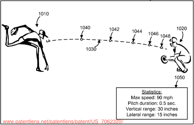
Scraping with pitchRx

library(pitchRx)
dat <- scrapeFX(start="2008-01-01", 
                end="2013-01-01")
atbats <- dat$atbat
pitches <- dat$pitch

Advanced Scraping

• scrapeFX can return up to seven different data frames

dat <- scrapeFX(start="2008-01-01", 
                end="2013-01-01"
                tables = list(atbat = NULL, 
                              pitch = NULL,
                              coach = NULL, 
                              runner = NULL, 
                              umpire = NULL, 
                              player = NULL, 
                              game = NULL))

• The function urlsToDataFrame can be used to manipulate any collection of XML files into a list of data frames.

Strike-zone plots

1. Strike-zone plots have height of the batter on the vertical axis and data points correspond to the location of baseballs as they cross home plate.
2. pitchRx can easily produce two types of strikezone plots:

• frequencies
• probabilities of events (more interesting in most cases)

3. Useful for answering questions such as: Do umpires favor home (as opposed to away) pitchers?

• More specifically: Given the umpire has to make a decision, do home pitchers have a higher chance of receiving a called strike?"

Some terminology

• A called strike is a case where the batter does not swing and the umpire declares the pitch a strike (which is a favorable outcome for the pitcher).

• A ball is an instance where the batter doesn’t swing and the umpire declares the pitch a ball (which is a favorable outcome for the batter).

• By restricting ourselves to these two outcomes, we condition upon a situation where the umpire has to make a binary decision about the pitch.

Probability of a Called Strike

• Here we use gam from the mgcv package to visualize the probability of a called strike (given the ump has to make a decision).

pitchFX <- plyr::join(dat$pitch, dat$atbat, 
                by=c("num", "url"))
decisions <- subset(pitchFX, des %in% 
                    c("Called Strike", "Ball"))
decisions$strike <- as.numeric(decisions$des == 
                                 "Called Strike")
strikeFX(decisions, model=gam(strike~s(px)+s(pz), 
          family = binomial(link='logit')), 
          layer=facet_grid(.~stand))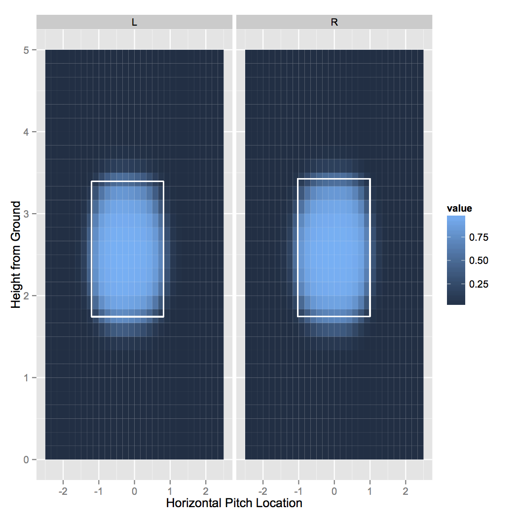

Difference in probability of Called Strike

• We can also visualize the difference in probabilistic events by adding arguments to density1 and density2.

• Here we find the probability of a called strike during the top inning minus the probability of a called strike during the bottom inning (top inning == home pitcher).

strikeFX(decisions, model=gam(strike~s(px)+s(pz), 
          family = binomial(link='logit')), 
          density1=list(top_inning="Y"), 
          density2=list(top_inning="N"), 
          layer=facet_grid(.~stand))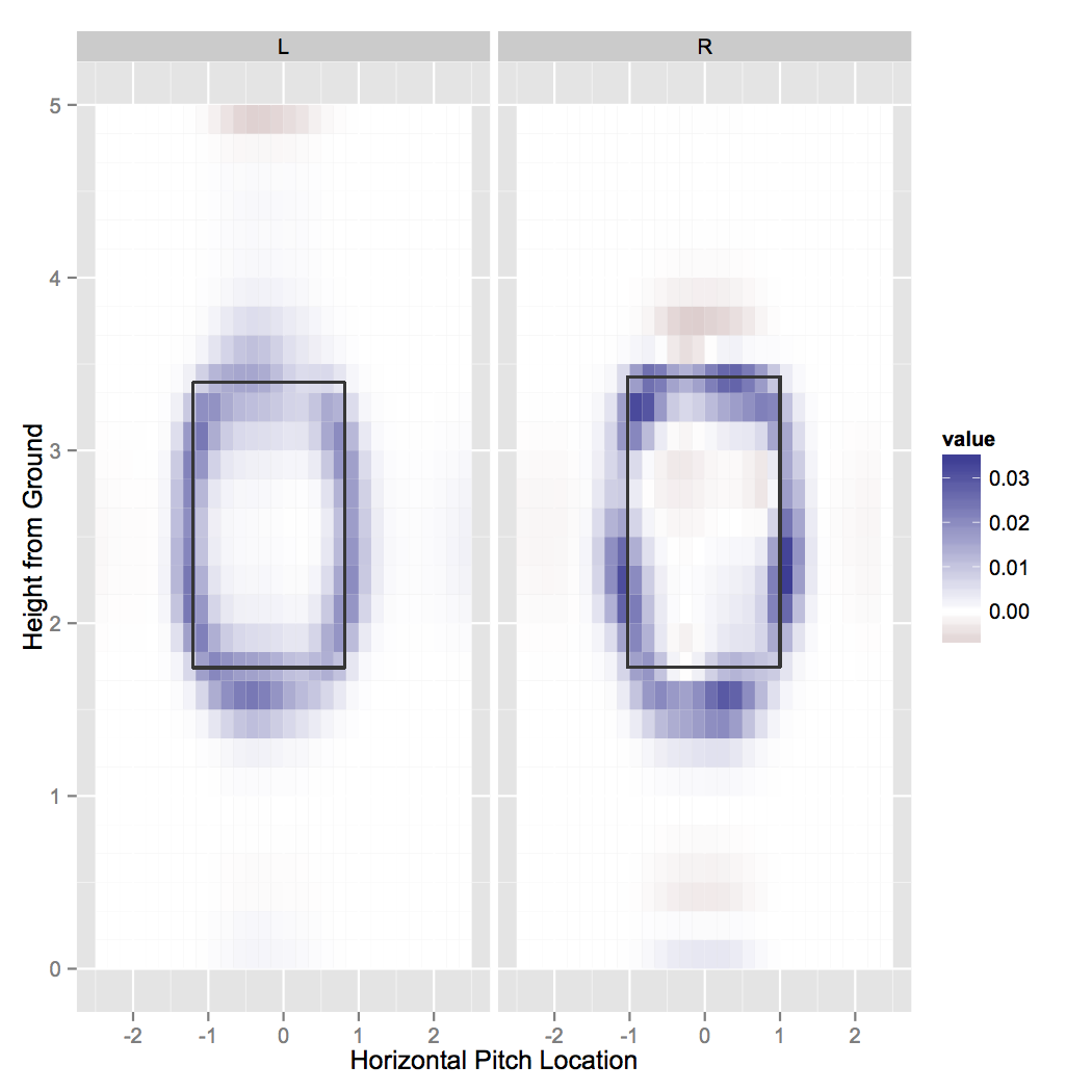

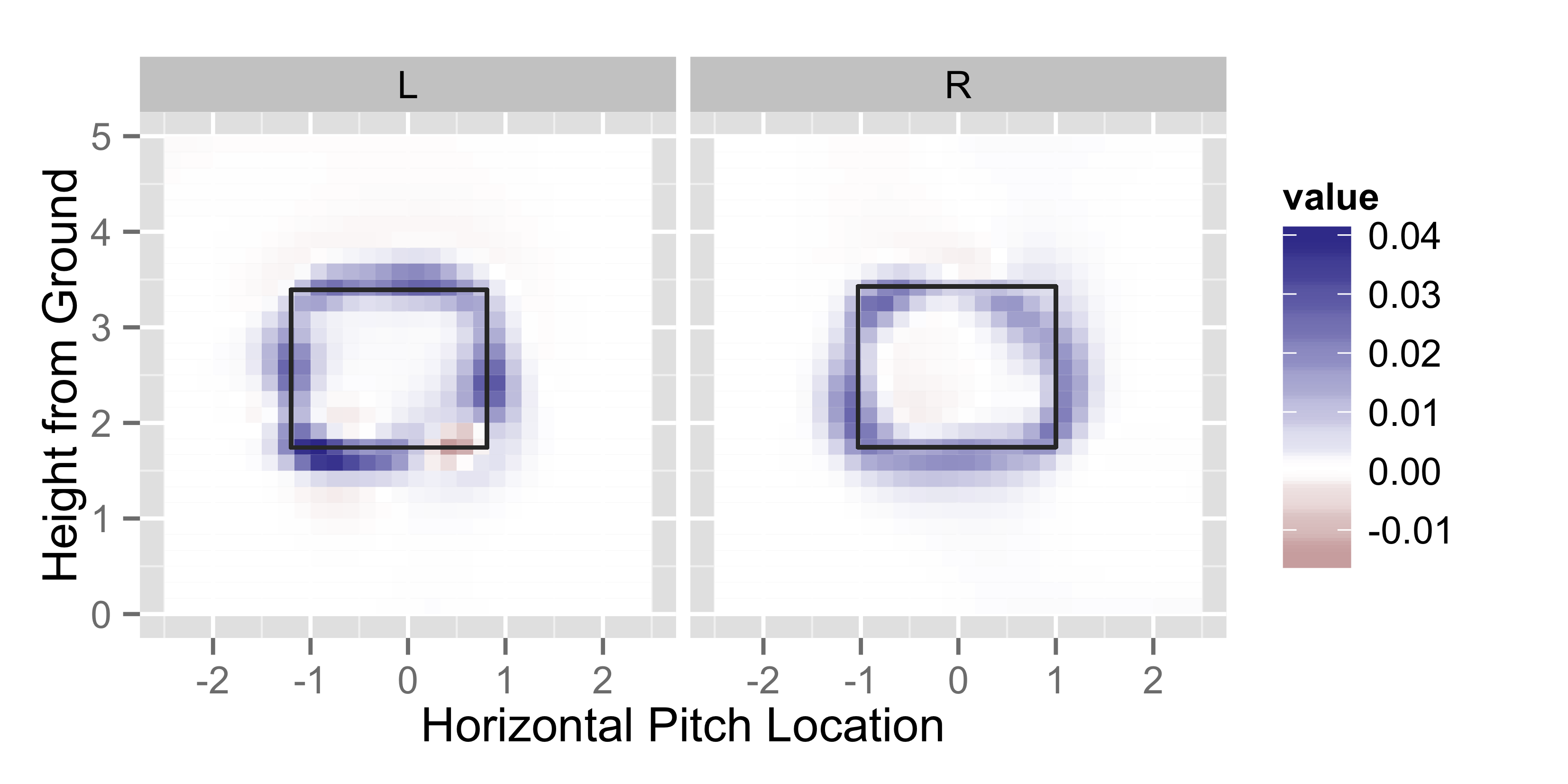
Home Field Advantage

• It appears away teams actually have something valid to complain about…

Strike-zones vs Trajectories

• strikeFX is nice for visualizing a lot of data (we just visualized over 1.5 million pitches).

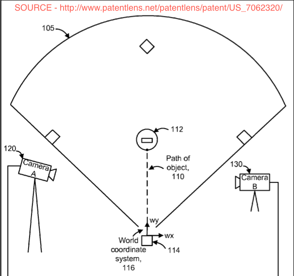
• PITCHf/x can also be used to regenerate (approximate) pitch trajectories.

• It isn’t straightforward to animate millions of pitch trajectories, so we usually restrict our focus to a few cases.

Yu Vishnu Darvish - a case study

*Created by Drew Sheppard @DShep25

Get the data

dat <- scrapeFX(start="2013-04-24", 
                end="2013-04-24")
atbats <- subset(dat$atbat, 
                 pitcher_name == "Yu Darvish")
Darvish <- plyr::join(atbats, dat$pitch, 
                by=c("num", "url"), type="inner")

• Darvish contains info on every pitch thrown by Yu Darvish on April 24th, 2013.

PITCHf/x animation

• animateFX can be used in a similar fashion to strikeFX for producing a series of plots that track pitch locations over time.

• As the animateFX animations progress, the pitches are being thrown directly towards you.

animateFX(Darvish, layer=list(theme_bw(),
                    coord_equal(),
                    facet_grid(.~stand)))

Real time animation

Whoa, nelly!!!

• Real time animations are hard to digest!

• Plotting that many pitches makes it even worse…

Normalized PITCHf/x

• Let’s average over pitch type (to get a typical flight path)

animateFX(Darvish, avg.by="pitch_types", 
          layer=list(coord_equal(),
          theme_bw(),
          facet_grid(.~stand)))

Normalized animation

WebGL Graphics

RH <- subset(Darvish, stand=="R")
interactiveFX(RH, avg.by="pitch_types")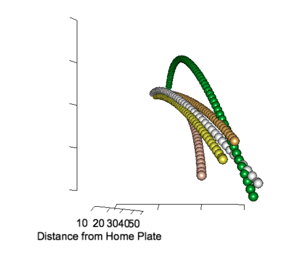

Want more??

1. Visit the pitchRx demo page (now included with CRAN package as R Markdown vignette).
2. R Journal article coming soon!
3. My web app.

• Slick user interface to strikeFX and animateFX
• Upload your own csv files!

4. Contribute to development or post an issue on GitHub.
5. I occasionally blog and tweet @cpsievert about pitchRx.

Special Thanks to:

This project wouldn’t be possible without the help of these people/organizations. Thank you for your help and/or great work!!!

• Heike Hofmann (my major professor) @heike_hh
• Di Cook @visnut
• Yihui Xie @xieyihui
• Ramnath Vaidyanathan @ramnath_vaidya
• RStudio @rstudioapp
• Hadley Wickham @hadleywickham
• Joe Cheng @jcheng
• Winston Chang @winston_chang
• MLB Advanced Media @mlbdotcom
• Alan Nathan @pobguy
• Mike Fast @fastballs
• Brian Mills @BMMillsy

Thanks for listening!